The Joys of Tangled Power Cables: Discrete Elastic Rods

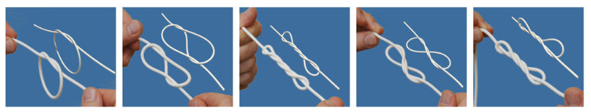
Find a cable (the power cable of your computer, or a headphone cable, will do nicely). Take hold of it from two points, about a hand’s breadth apart. Try twisting, bending, and pulling it. Notice how it resists your efforts. Notice how the cable has a natural bend and twist to it, even at rest. Notice also how, when slowly twisted, the cable will stay mostly stationary, building up tension, before springing into some new stable state. If the cable is long or flexible enough, you might be able to make it form twisty loops that hang off the main span. This paper attempts to model these behaviours.

This seems daunting: the behaviours displayed are complex, and the relationship between the external forces and the final state is hard to intuit. But there is a classic trick for modeling flexible objects like the power cable. The idea is to define the energy built up within the object as a function of the object’s position and deformation.

E = E(γ)

As long as such a function can be defined, the resulting forces can be found as the gradient of the energy with respect to the positions – in other words, what direction would some small part of the cable have to be perturbed to decrease the energy. That small part will then feel a force in that direction.

F = ∇E

Once we have forces, we can plug them into Newton’s famous second law

F = ma

d²γ/dt² = F/m

This gives us the acceleration of the cable. From the acceleration, we can adjust the velocities, and from the velocities the positions. The new positions will give a new gradient for the energy, and thus new forces, and so on. So, the bulk of the thinking is just finding the energy function E.

But first we must have some way of representing the cable’s position. Now real power cables are complicated objects, made of many materials with different properties. This paper makes some assumptions about the objects modeled.

• The cable is inextensible – no matter how hard it is pulled, it will not get any longer. The length of the whole cable or of any sub-section of it is constant
• The cable is elastic – it has a constant rest position it will always try to return to. If a real cable is bent hard or kept in a bent position for a long time, its rest position will change and it will become permanently bent. We will assume this cannot happen
• The cable’s resistance to bending and twisting is linear. The great physicist Hooke (a life-long rival of that cad Isaac Newton) showed that the force exerted by a stretched metal cable is proportional to the amount it is stretched. We will assume our rod works the same way: its force will be proportional to the amount it is bent or twisted. Note that the cable might be more or less resistant to bending depending on the axis along which it is bent – a cable that is wide and flat like a ribbon might bend easily out of its plane but be much stiffer in its plane.

Fun With Linear Algebra

The variables defined in the creation of the energy function are a terrific exercise in three-dimensional linear algebra. Let us start with our position variable, γ.

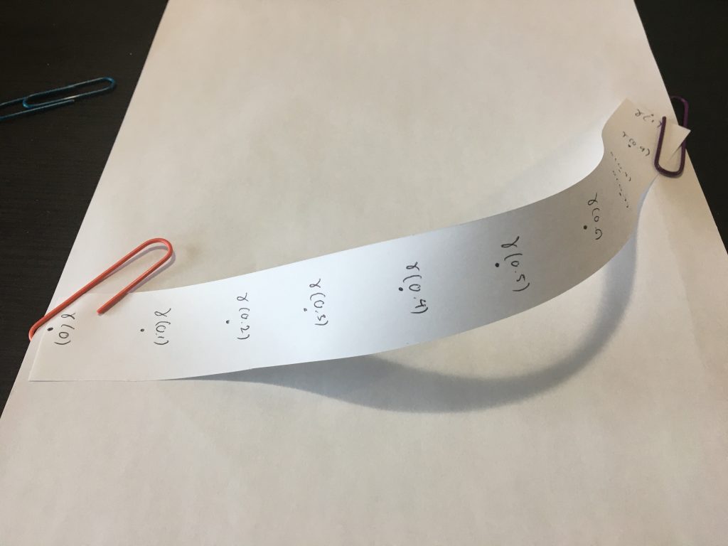
γ is a function of s, where s is a measure of distance along the cable. So s = 0 means one end of the cable, s = 1 is the other end, s = 0.5 is the exact middle, and so on. Note that since the cable is of fixed length, each value of s points unambiguously to one point along the cable. γ, our first variable, is just the position of that point.

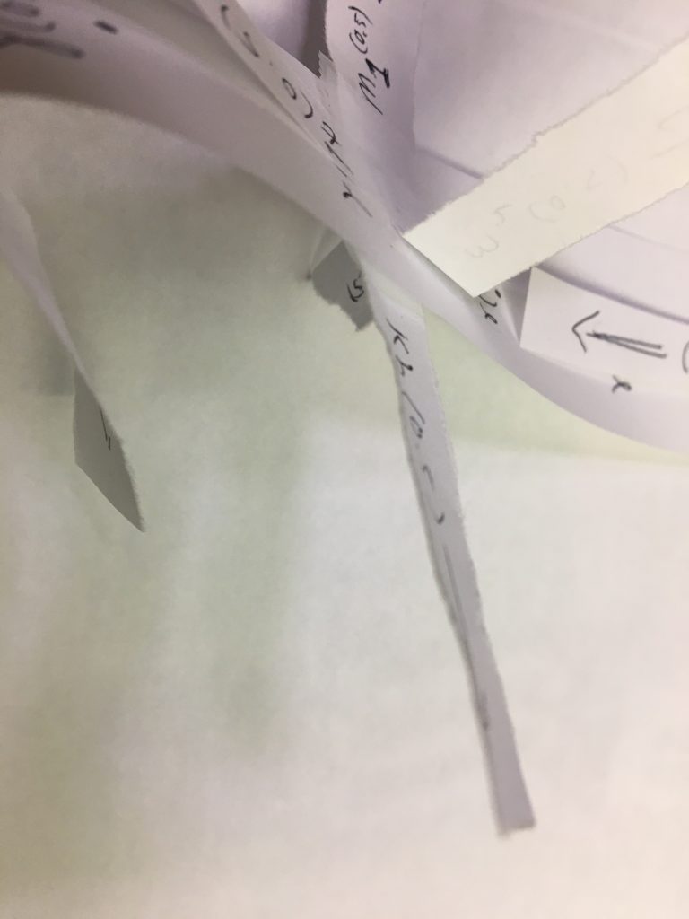
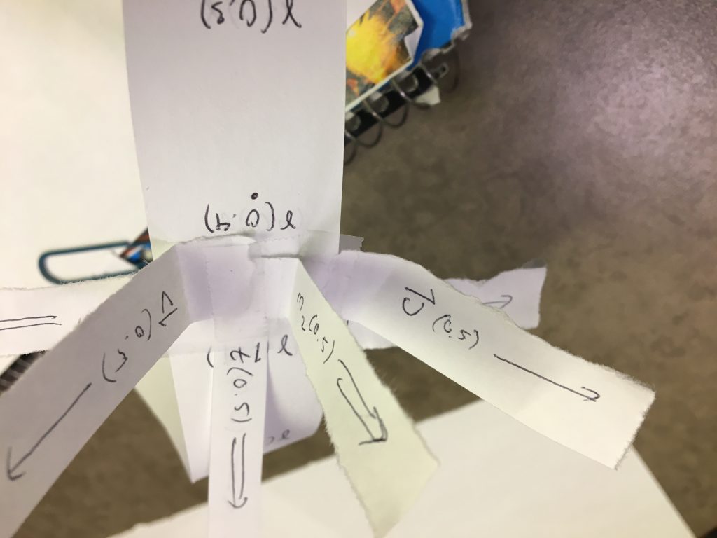
Here are some γ’s marked on an elastic rod

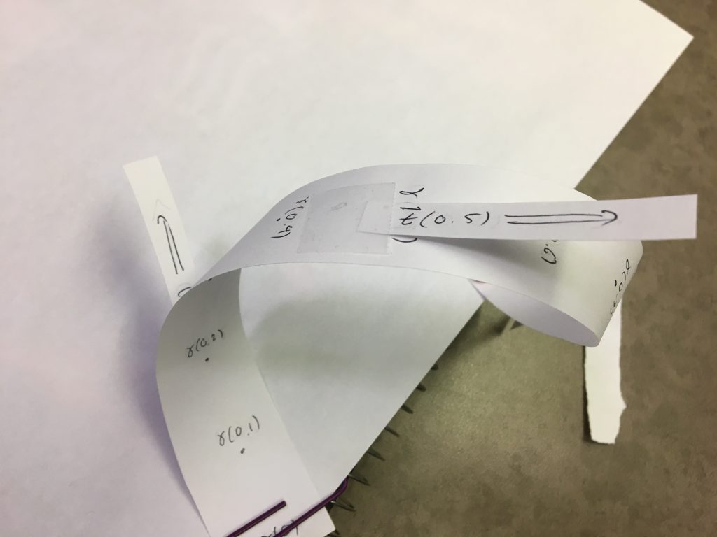
Our next variable is t. t is a vector pointing along the cable, parallel to it, in the positive s direction. Numerically, it is defined as

t = dγ/ds

That makes sense, as t is the direction in which gamma is “moving” as we increase s. Once again, since the cable is inextensible, t is of constant magnitude: we may assume that constant magnitude is 1.

t is most easily visualized as attached to the elastic rod along its length: paper clips can work but they affect the shape of the rod, so tape is better.

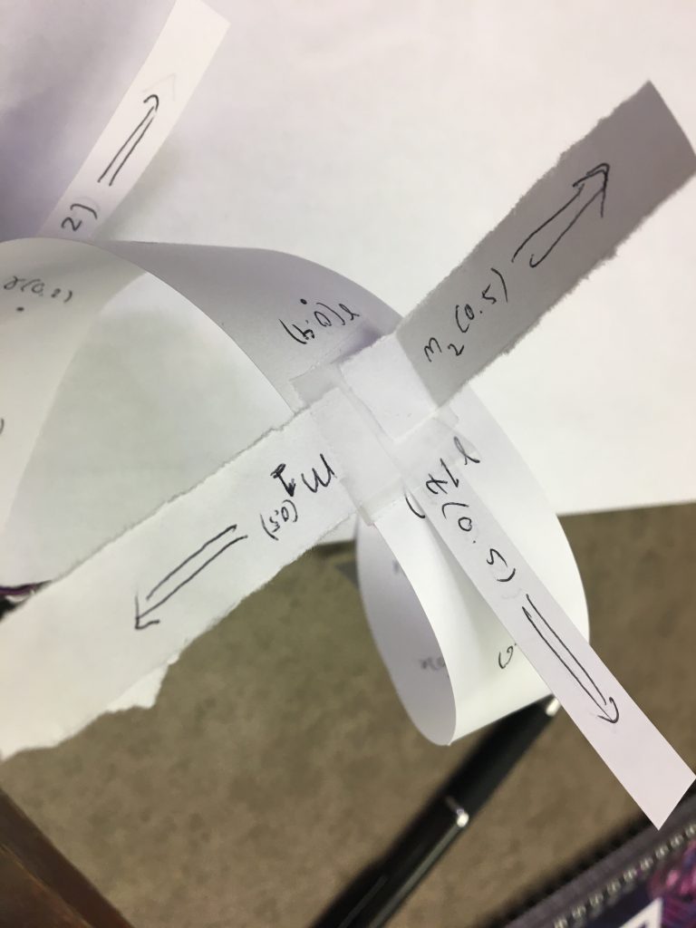
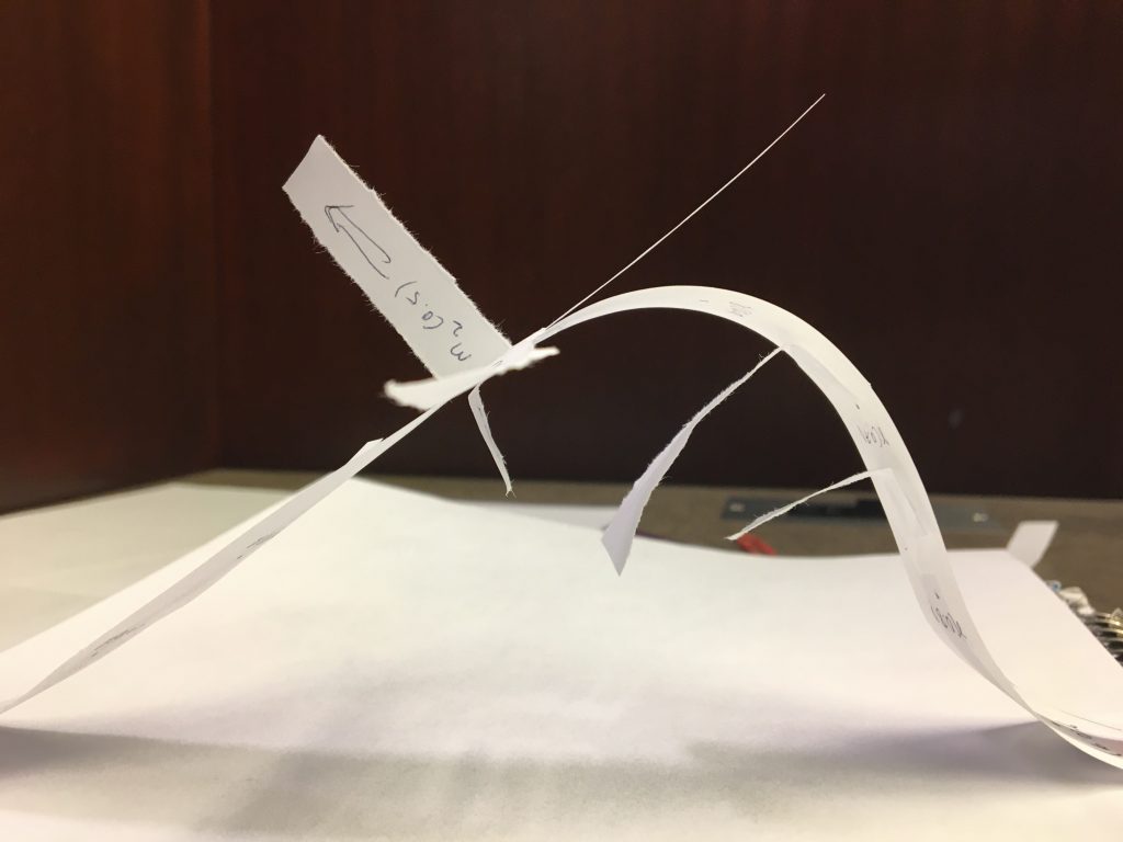
m₁ and m₂ are two vectors that are perpendicular to each other and to t. Together they define a plane that the cable is pointing straight out of (t is the normal of that plane). They indicate the twisting of the cable, i.e. if the cable was coloured differently on its two sides, m₁ would always point out of the same side.

κ is the curvature of the wire: it is a vector pointing into the direction the wire is curving, and its magnitude is greater the tighter the curve. Numerically, κ is the rate of change of t.

κ = dt/ds

The best part about 3-d linear algebra is making shapes with your hands: see if you can visualize how t rotates as the rod curves, and the direction it rotates – κ – points into the curve.

We now have all we need to define the bending energy. kappa is perpendicular to t (can you see why?), and so it lies in the m₁-m₂ plane. Because the bending force might be stronger or weaker depending on whether it is in the m₁ or m₂ direction, we can break down kappa into two parts.

ω₁ = κ ⋅ m₁ ω₂ = κ ⋅ m₂

By integrating omega1 and omega2, we can get the bending energy

E_bending = ∫B₁ω₁²ds + ∫B₂ω₂²ds

Where B₁ and B₂ describe the resistance to bending in the m₁ and m₂ directions

The twisting is a little trickier. How do we measure the twisting of a curve that is also bending?

First, we’re going to need one more variable, κb.

κb = t ⨯ κ = t ⨯ dt/ds

κb is perpendicular to both t and κ. If the curve around γ(s) is in a plane, κb is normal to that plane. Since κb is perpendicular to t, it is also in the m₁-m₂ plane.

Now we can define our last two variables, u and v. u and v are the rest twist: they are what m₁ and m₂ would be if there was no twisting, but the cable maintained its same path γ(s). u and v are perpendicular to each other and to t, and the formula is

u ⋅ κb = du/ds v ⋅ κb = dv/ds

Try to convince yourself that this is right, that if we had m₁ = u and m₂ = v, then the cable would have no twist in it.

Now u and v, although they are not equal to m₁ and m₂, are in the m₁-m₂ plane. So we can define θ as the angle between u and m₁. θ measures how much the twisting of the curve at any point differs from the rest case with no twisting. If θ is changing, the cable must be twisting

E_twisting = ∫T(dθ/ds)²ds

With T being the local resistance to twisting, and

E = E_bending + E_twisting

the total energy.

Extra details

That isn’t quite everything, though it is all of the interesting stuff. Here are some minor details I have to mention.

• The object might have some amount of rest bending, so the bending energies need to be tweaked somewhat to take that into account.
• The forces that come out of these energies might result in the cable getting longer or shorter or intersecting itself. Additional constraints must be added to the simulation to prevent those things happening.
• Instead of using strips of paper, the writers of this paper used a computer. Because of this, they had to represent the position of the elastic rod as a series of discrete points instead of a continuous curve. This requires modification to all the mathematics: all the integrals become sums and everything is much less pretty.

And with just that, this paper manages to simulate cables that match up with reality remarkably well

Thanks for reading!