It’s Summer 1999! Nunavut is the newest Canadian province, the Euro is here, some guy called George W. Bush says he’s running for President (like he has any chance!) and George Lucas just released the first prequel to his Star Wars franchise (I haven’t seen it yet, but I assume it’s just as good as the others!)
It’s an exciting time to live in the world, and it is made even more exciting by the latest leap in realistic fluid simulation carried out by the newest SIGGRAPH paper Stable Fluids.
Here’s the thing. When you see fluids like smoke or water in an animated movie or videogame, chances are they have been animated manually by an artist, usually from a set of predetermined motions that the artist combines. This has many problems: first, as you may have noticed, it does not always lead to the most realistic animations! And second, it takes up a lot of effort and time that could be spent elsewhere.
So, if manually animating a fluid is really expensive and unrealistic, what other option do we have? The obvious answer is we could use real fluids; i.e., using special effects instead of computer-generated fluids. This would be simple: we would just need to place some fluid in an initial configuration (for example, start up a chimney generating smoke), and record how it moves and propagates as it follows the laws of physics in the real world. We could add some physical constraints: for example, place the chimney inside a box from which the smoke cannot escape. When we set up a scene like this in the real world, there is no artist deciding each movement of the fluid: rather, some initial conditions and constraints are set up, and physics takes care of the rest. In a way, physics becomes the artist.
You may already be thinking: “well, why don’t we do just that, but virtually?” Let’s model the physical scene we want to set up in a computer, specify mathematically constraints and initial conditions, translate the physical rules of the real world into rules for how our models behave in the virtual world, and record what comes out! This means, instead of manually modelling the fluid, we can physically simulate it: We can represent a fluid; for example, as particles on a computer or as a volume density, and we can make sure that they satisfy the physical equation governing fluids in the real world, known as the Navier-Stokes equation:
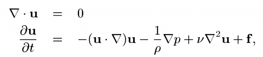
Solving this equation gives us a velocity map, which we can then use to see the direction and speed with which any particle moves. Once we have that velocity, we can choose a tiny timestep and move each particle according to that velocity, to then solve the equation again, etc.
So that’s it! Problem solved! … Well, not quite. What we described above is called an explicit simulation, which just means each particle is moved according to the velocity it has at the moment it starts the movement. Of course, in real life, that velocity would change as the particle is displaced; and, by using only the velocity at the start of the movement, we are assuming some error. This error can compound and eventually make our simulation explode and return absurd values.
“But what if we make the timestep really really tiny? The velocity cannot change too much then“, you may be thinking. And you would be right! But if our timestep is super super small, then we will need to solve the equation many many times, and that comes with a massive performance cost. So, in explicit simulations, the choice is between risking blowing up or taking a big blow to the speed at which our code runs.
What can we do then? We could do what’s called an implicit simulation. This is slightly more complicated: instead of moving each particle by its velocity at the current time, we move each particle by the velocity it will have after moving. Of course, we don’t know the velocity it will have after moving until after we have moved it, so there is no way to compute that directly. Instead, we need to link these two unknowns and solve an equation to compute the new position of each particle. This method allows much larger timesteps than explicit ones, but solving this new equation takes time, so the gain isn’t as big. It also has other problems: instead of blowing up, it can now dampen the simulation and it is usually much more complicated to code.
So, is that really the choice? Explosions and bad performance versus damping, slightly better performance and hard implementations? Well, yes, it is! Or rather… it was, until the recent arrival of Stable Fluids. We will not go deep into the math of the paper but, basically, the contribution is using not the velocity at the current timestep, and not the velocity at the next timestep; instead, the velocity at the previous timestep. This apparently simple contribution means the simulation is guaranteed not to blow up, and it is simple to implement (we surely have already computed the velocity in the previous timestep). It is then, in a way, the best of both worlds.
So there you go! Amazing, fast, stable, simple to implement fluid simulations! This can revolutionize the simulations we see in movies and video games! I am excited to see it at work in the The Fast and The Furious, the new movie apparently currently in the works. I hope it has a very detailed, elaborate plot!