WRAPD: Weighted Rotation-aware ADMM for Parameterization and Deformation

Motivation

Recently, there has been a tendency toward optimization formulation in computer graphics, and as a result, designing robust and fast solvers for this purpose has become a hot topic among researchers. There are numerous methods that optimizers utilize for solving an optimization problem, and Newton’s method is one of the most famous ones.

The main bottleneck in Newton’s method is solving a system of linear equations in each iteration, and various methods have tried to evade solving this system accurately using approximations of the Hessian information of the objective function (including the possible barrier terms).

On the other hand, there are methods such as ADMM that are less computationally expensive and have shown fast convergence behaviour in many applications. But such solvers may suffer from slow convergence in the early iterations, and in this article, some solutions to these problems are discussed.

Before proceeding to the main bottlenecks of the available methods and trying to improve them, let’s have a review of the available local-global solvers and get more familiar with the notations used throughout this article.

Local-global Solvers in Computer Graphics

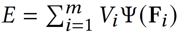
Let’s assume that we have n nodes with m elements in R^d where d can take values in set {2, 3}, and the possible elements are springs, triangles, or tetrahedra. If x_i shows the position of node i, then we can define the position matrix X = [x₁,x₂,…,x_n]^T and it is clear that the deformation gradient is a linear function of the node positions. As a result, the deformation gradient can be formulated as F_i = (D_i X)^T, where D_i is in R^kxdwhere k can take the value of 1 for springs, 2 for triangles, and 3 for tetrahedra.

Using the notations introduced above, the total energy of the model can be formulated as follows:

Our goal is to minimize the energy of the system, and as a result, this minimization problem can be formulated as follows:

where we have defined C_i= (D_i X)^T – Z_i. For solving this minimization problem, the associated augmented Lagrangian function is constructed as shown below (for more information about the derivation, please check the supplementary material provided here):

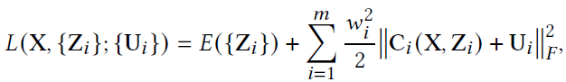
where w_i is the scalar weights for i^th element.

This optimization problem can be solved iteratively with three steps in each iteration:

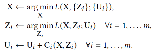
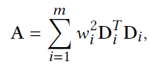
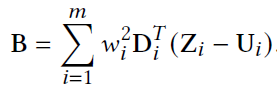
Considering the linear coupling constraints in the model, the optimization problem that yields the value of X is a quadratic function of X, and as a result, can be solved using a single iteration of Newton’s method, which includes a single linear solve to some system AX = B. The good feature about this system is the fact that A is a constant matrix as shown below, and can be prefactorized once and used in multiple iterations of the solving.

Also, the computation of the right-hand side is not so expensive, as B is the summing contributions from all elements of the system as shown below:

Solving for Z_i‘s can also be performed in parallel, as different Z_i‘s are independently found. Efficient implementations of these small-scale problem solves on CPU or GPU, in addition to the proper prefactorization for the matrix A can result in a quite efficient solution to the energy minimization problem introduced earlier.

Limitations of Local-global Solvers

The aforementioned method for solving problems with linear coupling constraints looks quite efficient, but still, there are some downsides to this method that can be improved. Two of the most profound limitations of this method that are addressed in this article will be briefly discussed below.

The first issue with the method is that the gradient deformation is a rotation-dependent measure. This fact shows its degrading impact when the initial guess to the optimal solution has a large rotational difference since the rotation of each element is updated during multiple iterations of global and local solves. In the paper, it is shown that even mild amounts of element rotations may hinder the convergence.

The other problem with this method is that the speed of convergence of the solver is highly dependent on the weight values w_i‘s. The importance of weights is so high that a poor choice of weights may make the algorithm not converge. Finding the proper weights for the problem is quite hard, and this can be considered as one of the downsides of the local-global solvers.

In the following sections, some possible solutions to the mentioned limitations are proposed.

Rotation-aware ADMM

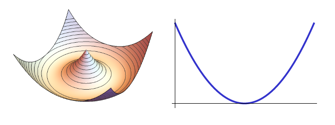
The local coordinates used earlier were translation-invariant, but they were sensitive to rotation. To address the first issue discussed earlier, one can try to find rotation-invariant local coordinates. This is done by using the polar decomposition of the deformation gradient F_i=R_iS_i, and only using the symmetric factor S_i inside the energy functions.

This choice of local coordinates helps make energy functions much more well-behaved, for example by using the rotation-invariant part of the coordinates, one can even make the spring energy function a convex function (see below figure).However, this choice of local coordinates will make the objective function in the global step nonlinear (but still smoothly defined).

By noting the fact that from the perspective of rotationally-invariant deformation energies, F_i and sym(F_i) are the same, one can try to solve the main optimization problem using the constraints in the new coordinates. The results of this modification doesn’t change much in the way the problem is solved (you can substitute C_i with C_i^sym= sym((D_i X)^T) – Z_i in the formulations of the previous section).

In the global step, the following problem is solved:

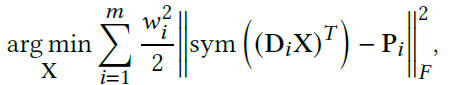
where P_i=Z_i-U_i. L-BFGS can be used for solving this minimization problem. In L-BFGS, a low-rank approximation of the Hessian matrix is computed (and modified) in every iteration.

The speed of the convergence of the system is dependent on the time spent on both the global step and the local step, and since L-BFGS is only utilized in the global step, running it for a large number of iterations won’t solely make the ADMM converge faster. Indeed, in case of having many non-rotational material deformations, running the local step frequently plays a paramount role in the convergence.

Dynamic Reweighting

As discussed earlier, the weights play a significant role in the convergence speed of the system. More specifically, lower weights will help the solver take larger steps, while puting the convergence at stake, while small weights will have an opposite effect on the solver. Currently, simple heuristics are used for tuning the weights, but they usually don’t work well in case of highly deformed meshes.

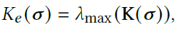
The heuristic used in this article is computing the weights from the maximum eigenvalue of the current Hessian of the system, i.e.

This idea has been previously used, but there are two main issues with the previous implementations.

Firstly, in case of highly deformed meshes in the beginning, the maximum eigenvalue will be extremely large, leading to small steps in the first iterations.

Secondly, as discussed earlier, one of the advantages of the local-global solvers is reusing the prefactorization of the matrix A in multiple iterations. But, by changing the weights in every iteration, the matrix A will be modified as well, resulting in new factorizations in each iteration.

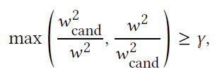
For solving the aforementioned issues, the following weighting scheme is used:

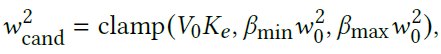
where cand shows the candidate weight, V₀ shows the volume of the system, and betas are user defined constants. Clamping the values is used for preventing small changes in the weights that will result to unnecessary modifications in the prefactorization of matrix A. After each global step, the current weights are compared to the candidate weights, and in case a weight satisfies the following constarint, in which gamma is a user-defined constant, the weights are updated, the U_i variables are scaled for consistency, and the matrix A is refactorized, following clearing the L-BFGS history.

Conclusion

In this article, after having an overall review of the local-global solvers in computer graphics, two main issues in them are analyzed, and in a detailed discussion, separate solutions to each of them are proposed.

The algorithm proposed in the paper outperforms state-of-the-art solvers in computer graphics, and except for a few constant, there is no need to tune parameters (such as the weights).

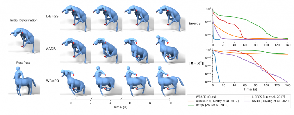
We conclude this article by an image of the main paper, comparing different solvers in time.

Thank you for your attention!